Spyctral’s Tutorial

This tutorial is a guide to use Spyctral package. Here we show, step by step, how to get started and the principal available options.

Install the library

!pip install spyctral-tools

Collecting spyctral-tools
  Using cached spyctral_tools-0.0.1rc0-py3-none-any.whl.metadata (6.4 kB)
Requirement already satisfied: attrs in /home/ccerdosino/anaconda3/envs/spyctral/lib/python3.13/site-packages (from spyctral-tools) (25.1.0)
Collecting numpy (from spyctral-tools)
  Using cached numpy-2.2.3-cp313-cp313-manylinux_2_17_x86_64.manylinux2014_x86_64.whl.metadata (62 kB)
Requirement already satisfied: python-dateutil in /home/ccerdosino/anaconda3/envs/spyctral/lib/python3.13/site-packages (from spyctral-tools) (2.9.0.post0)
Collecting astropy (from spyctral-tools)
  Using cached astropy-7.0.1-cp313-cp313-manylinux_2_17_x86_64.manylinux2014_x86_64.whl.metadata (10 kB)
Collecting pandas (from spyctral-tools)
  Using cached pandas-2.2.3-cp313-cp313-manylinux_2_17_x86_64.manylinux2014_x86_64.whl.metadata (89 kB)
Collecting specutils (from spyctral-tools)
  Using cached specutils-1.19.0-py3-none-any.whl.metadata (6.0 kB)
Collecting matplotlib (from spyctral-tools)
  Using cached matplotlib-3.10.0-cp313-cp313-manylinux_2_17_x86_64.manylinux2014_x86_64.whl.metadata (11 kB)
Collecting pyerfa>=2.0.1.1 (from astropy->spyctral-tools)
  Using cached pyerfa-2.0.1.5-cp39-abi3-manylinux_2_17_x86_64.manylinux2014_x86_64.whl.metadata (5.7 kB)
Collecting astropy-iers-data>=0.2025.1.31.12.41.4 (from astropy->spyctral-tools)
  Using cached astropy_iers_data-0.2025.2.24.0.34.4-py3-none-any.whl.metadata (5.1 kB)
Requirement already satisfied: PyYAML>=6.0.0 in /home/ccerdosino/anaconda3/envs/spyctral/lib/python3.13/site-packages (from astropy->spyctral-tools) (6.0.2)
Requirement already satisfied: packaging>=22.0.0 in /home/ccerdosino/anaconda3/envs/spyctral/lib/python3.13/site-packages (from astropy->spyctral-tools) (24.2)
Collecting contourpy>=1.0.1 (from matplotlib->spyctral-tools)
  Using cached contourpy-1.3.1-cp313-cp313-manylinux_2_17_x86_64.manylinux2014_x86_64.whl.metadata (5.4 kB)
Collecting cycler>=0.10 (from matplotlib->spyctral-tools)
  Using cached cycler-0.12.1-py3-none-any.whl.metadata (3.8 kB)
Collecting fonttools>=4.22.0 (from matplotlib->spyctral-tools)
  Using cached fonttools-4.56.0-cp313-cp313-manylinux_2_5_x86_64.manylinux1_x86_64.manylinux_2_17_x86_64.manylinux2014_x86_64.whl.metadata (101 kB)
Collecting kiwisolver>=1.3.1 (from matplotlib->spyctral-tools)
  Using cached kiwisolver-1.4.8-cp313-cp313-manylinux_2_17_x86_64.manylinux2014_x86_64.whl.metadata (6.2 kB)
Collecting pillow>=8 (from matplotlib->spyctral-tools)
  Using cached pillow-11.1.0-cp313-cp313-manylinux_2_28_x86_64.whl.metadata (9.1 kB)
Collecting pyparsing>=2.3.1 (from matplotlib->spyctral-tools)
  Using cached pyparsing-3.2.1-py3-none-any.whl.metadata (5.0 kB)
Requirement already satisfied: six>=1.5 in /home/ccerdosino/anaconda3/envs/spyctral/lib/python3.13/site-packages (from python-dateutil->spyctral-tools) (1.17.0)
Collecting pytz>=2020.1 (from pandas->spyctral-tools)
  Using cached pytz-2025.1-py2.py3-none-any.whl.metadata (22 kB)
Collecting tzdata>=2022.7 (from pandas->spyctral-tools)
  Using cached tzdata-2025.1-py2.py3-none-any.whl.metadata (1.4 kB)
Collecting scipy>=1.3 (from specutils->spyctral-tools)
  Using cached scipy-1.15.2-cp313-cp313-manylinux_2_17_x86_64.manylinux2014_x86_64.whl.metadata (61 kB)
Collecting gwcs>=0.18 (from specutils->spyctral-tools)
  Using cached gwcs-0.24.0-py3-none-any.whl.metadata (6.3 kB)
Collecting asdf-astropy>=0.3 (from specutils->spyctral-tools)
  Using cached asdf_astropy-0.7.1-py3-none-any.whl.metadata (7.3 kB)
Collecting asdf>=2.14.4 (from specutils->spyctral-tools)
  Using cached asdf-4.1.0-py3-none-any.whl.metadata (14 kB)
Collecting ndcube>=2.0 (from specutils->spyctral-tools)
  Using cached ndcube-2.3.1-py3-none-any.whl.metadata (7.5 kB)
Collecting asdf-standard>=1.1.0 (from asdf>=2.14.4->specutils->spyctral-tools)
  Using cached asdf_standard-1.1.1-py3-none-any.whl.metadata (5.2 kB)
Collecting asdf-transform-schemas>=0.3 (from asdf>=2.14.4->specutils->spyctral-tools)
  Using cached asdf_transform_schemas-0.5.0-py3-none-any.whl.metadata (4.1 kB)
Collecting jmespath>=0.6.2 (from asdf>=2.14.4->specutils->spyctral-tools)
  Using cached jmespath-1.0.1-py3-none-any.whl.metadata (7.6 kB)
Collecting semantic_version>=2.8 (from asdf>=2.14.4->specutils->spyctral-tools)
  Using cached semantic_version-2.10.0-py2.py3-none-any.whl.metadata (9.7 kB)
Collecting asdf-coordinates-schemas>=0.3 (from asdf-astropy>=0.3->specutils->spyctral-tools)
  Using cached asdf_coordinates_schemas-0.3.0-py3-none-any.whl.metadata (4.1 kB)
Collecting asdf_wcs_schemas>=0.4.0 (from gwcs>=0.18->specutils->spyctral-tools)
  Using cached asdf_wcs_schemas-0.4.0-py3-none-any.whl.metadata (3.9 kB)
Using cached spyctral_tools-0.0.1rc0-py3-none-any.whl (21 kB)
Using cached astropy-7.0.1-cp313-cp313-manylinux_2_17_x86_64.manylinux2014_x86_64.whl (10.3 MB)
Using cached numpy-2.2.3-cp313-cp313-manylinux_2_17_x86_64.manylinux2014_x86_64.whl (16.1 MB)
Using cached matplotlib-3.10.0-cp313-cp313-manylinux_2_17_x86_64.manylinux2014_x86_64.whl (8.6 MB)
Using cached pandas-2.2.3-cp313-cp313-manylinux_2_17_x86_64.manylinux2014_x86_64.whl (12.7 MB)
Using cached specutils-1.19.0-py3-none-any.whl (4.9 MB)
Using cached asdf-4.1.0-py3-none-any.whl (961 kB)
Using cached asdf_astropy-0.7.1-py3-none-any.whl (93 kB)
Using cached astropy_iers_data-0.2025.2.24.0.34.4-py3-none-any.whl (1.9 MB)
Using cached contourpy-1.3.1-cp313-cp313-manylinux_2_17_x86_64.manylinux2014_x86_64.whl (322 kB)
Using cached cycler-0.12.1-py3-none-any.whl (8.3 kB)
Using cached fonttools-4.56.0-cp313-cp313-manylinux_2_5_x86_64.manylinux1_x86_64.manylinux_2_17_x86_64.manylinux2014_x86_64.whl (4.8 MB)
Using cached gwcs-0.24.0-py3-none-any.whl (169 kB)
Using cached kiwisolver-1.4.8-cp313-cp313-manylinux_2_17_x86_64.manylinux2014_x86_64.whl (1.5 MB)
Using cached ndcube-2.3.1-py3-none-any.whl (137 kB)
Using cached pillow-11.1.0-cp313-cp313-manylinux_2_28_x86_64.whl (4.5 MB)
Using cached pyerfa-2.0.1.5-cp39-abi3-manylinux_2_17_x86_64.manylinux2014_x86_64.whl (738 kB)
Using cached pyparsing-3.2.1-py3-none-any.whl (107 kB)
Using cached pytz-2025.1-py2.py3-none-any.whl (507 kB)
Using cached scipy-1.15.2-cp313-cp313-manylinux_2_17_x86_64.manylinux2014_x86_64.whl (37.3 MB)
Using cached tzdata-2025.1-py2.py3-none-any.whl (346 kB)
Using cached asdf_coordinates_schemas-0.3.0-py3-none-any.whl (33 kB)
Using cached asdf_standard-1.1.1-py3-none-any.whl (81 kB)
Using cached asdf_transform_schemas-0.5.0-py3-none-any.whl (275 kB)
Using cached asdf_wcs_schemas-0.4.0-py3-none-any.whl (45 kB)
Using cached jmespath-1.0.1-py3-none-any.whl (20 kB)
Using cached semantic_version-2.10.0-py2.py3-none-any.whl (15 kB)
Installing collected packages: pytz, tzdata, semantic_version, pyparsing, pillow, numpy, kiwisolver, jmespath, fonttools, cycler, astropy-iers-data, asdf-standard, scipy, pyerfa, pandas, contourpy, asdf-transform-schemas, matplotlib, astropy, asdf, asdf-coordinates-schemas, asdf_wcs_schemas, asdf-astropy, gwcs, ndcube, specutils, spyctral-tools
Successfully installed asdf-4.1.0 asdf-astropy-0.7.1 asdf-coordinates-schemas-0.3.0 asdf-standard-1.1.1 asdf-transform-schemas-0.5.0 asdf_wcs_schemas-0.4.0 astropy-7.0.1 astropy-iers-data-0.2025.2.24.0.34.4 contourpy-1.3.1 cycler-0.12.1 fonttools-4.56.0 gwcs-0.24.0 jmespath-1.0.1 kiwisolver-1.4.8 matplotlib-3.10.0 ndcube-2.3.1 numpy-2.2.3 pandas-2.2.3 pillow-11.1.0 pyerfa-2.0.1.5 pyparsing-3.2.1 pytz-2025.1 scipy-1.15.2 semantic_version-2.10.0 specutils-1.19.0 spyctral-tools-0.0.1rc0 tzdata-2025.1

Import packages

The first thing to do is import the necessary libraries. In general, you will need the following:

• spyctral: the library that we present in this tutorial.

• numpy: to manipulate arrays.

• matplotlib.pyplot: to create and customize a wide range of static, animated, and interactive plots.

• os: to interact with the operating system, such as handling file paths and managing directories.

• csv: to read and write CSV files, which are commonly used for storing tabular data.

Note: In this tutorial, we assume that you already have experience using these libraries.

import spyctral as spy
import numpy as np
import os
import csv
import matplotlib.pyplot as plt

Load the data

Next step is load the data. Spyctral needs a minimum of one text file and you need to know the source code of the file to be analysed to use the correct read function.

The file path is the only mandatory setting in read functions and you must be sure to incluide the correct file/files path. You can also include extra configuration like asign the object name or the ammount of decimals to get the parameters values. Explore all the different options for each read function with help task to adapt it to your needs.

Single loading

For this tutorial step we will use a data file available in test folder for your try as well.

star_object_1 = spy.read_fisa('../../tests/datasets/case_SC_FISA.fisa')

star_object_2 = spy.read_starlight('../../tests/datasets/case_SC_Starlight.out', object_name='object_2')

Those lines created two SpectralSummary objects that store all the information from FISA and STARLIGHT files. Here we show the objects and how they save the data.

star_object_1

<SpectralSummary(
  header={fisa_version, date_time, reddening, adopted_template, normalization_point, spectra_names},
  data={Unreddened_spectrum, Template_spectrum, Observed_spectrum, Residual_flux},
  age, reddening, av_value, normalization_point, z_value,
  spectra={Unreddened_spectrum, Template_spectrum, Observed_spectrum, Residual_flux},
  extra_info={str_template, name_template, age_map, error_age_map, z_map})>

star_object_2

<SpectralSummary(
  header={Date, Cid@UFSC, arq_obs, arq_base, arq_masks, arq_config, N_base, N_YAV_components, i_FitPowerLaw, alpha_PowerLaw, red_law_option, q_norm, l_ini, l_fin, dl, l_norm, llow_norm, lupp_norm, fobs_norm, llow_SN, lupp_SN, S_N_in_S_N_window, S_N_in_norm_window, S_N_err_in_S_N_window, S_N_err_in_norm_window, fscale_chi2, idum_orig, NOl_eff, Nl_eff, Ntot_cliped, clip_method, Nglobal_steps, N_chains, NEX0s_base, Clip_Bug, RC_Crash, Burn_In, n_censored_weights, wei_nsig_threshold, wei_limit, idt_all, wdt_TotTime, wdt_UsrTime, wdt_SysTime, chi2_Nl_eff, adev, sum_of_x, Flux_tot, Mini_tot, Mcor_tot, v0_min, vd_min, AV_min, YAV_min, Nl_obs},
  data={synthetic_spectrum, synthetic_results, results_average_chains_xj, results_average_chains_mj, results_average_chains_Av_chi2_mass},
  age, reddening, av_value, normalization_point, z_value,
  spectra={synthetic_spectrum, observed_spectrum, residual_spectrum},
  extra_info={xj_percent, age_decimals, rv, z_decimals, ssps_vector, synthesis_info, average_log_age})>

Set loading

If you have a set of files, you can load all the files at once. To make that you can define the files list and their folder path. For example we select a set of 15 STARLIGHT files, and we save the objects from each file in a dictionary ss_objects.

folder_files_path ='../../tests/datasets/set_STARLIGHT_files'

files_list  = [f for f in os.listdir(folder_files_path) if os.path.isfile(os.path.join(folder_files_path, f)) and f.endswith('.out')]

ss_objects = {}
for idx, file in enumerate(files_list):
    var_name = f"ss_obj_{idx}"
    ss_objects[var_name] = spy.read_starlight(f'{folder_files_path}/{file}', object_name=file)

len(ss_objects)

30

ss_objects['ss_obj_1']

<SpectralSummary(
  header={Date, Cid@UFSC, arq_obs, arq_base, arq_masks, arq_config, N_base, N_YAV_components, i_FitPowerLaw, alpha_PowerLaw, red_law_option, q_norm, l_ini, l_fin, dl, l_norm, llow_norm, lupp_norm, fobs_norm, llow_SN, lupp_SN, S_N_in_S_N_window, S_N_in_norm_window, S_N_err_in_S_N_window, S_N_err_in_norm_window, fscale_chi2, idum_orig, NOl_eff, Nl_eff, Ntot_cliped, clip_method, Nglobal_steps, N_chains, NEX0s_base, Clip_Bug, RC_Crash, Burn_In, n_censored_weights, wei_nsig_threshold, wei_limit, idt_all, wdt_TotTime, wdt_UsrTime, wdt_SysTime, chi2_Nl_eff, adev, sum_of_x, Flux_tot, Mini_tot, Mcor_tot, v0_min, vd_min, AV_min, YAV_min, Nl_obs},
  data={synthetic_spectrum, synthetic_results, results_average_chains_xj, results_average_chains_mj, results_average_chains_Av_chi2_mass},
  age, reddening, av_value, normalization_point, z_value,
  spectra={synthetic_spectrum, observed_spectrum, residual_spectrum},
  extra_info={xj_percent, age_decimals, rv, z_decimals, ssps_vector, synthesis_info, average_log_age})>

ss_objects['ss_obj_14']

<SpectralSummary(
  header={Date, Cid@UFSC, arq_obs, arq_base, arq_masks, arq_config, N_base, N_YAV_components, i_FitPowerLaw, alpha_PowerLaw, red_law_option, q_norm, l_ini, l_fin, dl, l_norm, llow_norm, lupp_norm, fobs_norm, llow_SN, lupp_SN, S_N_in_S_N_window, S_N_in_norm_window, S_N_err_in_S_N_window, S_N_err_in_norm_window, fscale_chi2, idum_orig, NOl_eff, Nl_eff, Ntot_cliped, clip_method, Nglobal_steps, N_chains, NEX0s_base, Clip_Bug, RC_Crash, Burn_In, n_censored_weights, wei_nsig_threshold, wei_limit, idt_all, wdt_TotTime, wdt_UsrTime, wdt_SysTime, chi2_Nl_eff, adev, sum_of_x, Flux_tot, Mini_tot, Mcor_tot, v0_min, vd_min, AV_min, YAV_min, Nl_obs},
  data={synthetic_spectrum, synthetic_results, results_average_chains_xj, results_average_chains_mj, results_average_chains_Av_chi2_mass},
  age, reddening, av_value, normalization_point, z_value,
  spectra={synthetic_spectrum, observed_spectrum, residual_spectrum},
  extra_info={xj_percent, age_decimals, rv, z_decimals, ssps_vector, synthesis_info, average_log_age})>

Note: The next steps are available for all SpectralSummary, we make the showing with the second one for simplicity.

Getting data information

The created object contains several atributes and methods. You can obtain the object name, header information, spectra tables, age, reddening and other parameters. Here we show how to get some of them:

star_object_2.header

<header {'i_FitPowerLaw', 'arq_config', 'fobs_norm', 'red_law_option', 'AV_min', 'N_YAV_components', 'Nl_eff', 'idt_all', 'Cid@UFSC', 'clip_method', 'Flux_tot', 'arq_base', 'llow_norm', 'vd_min', 'Nglobal_steps', 'dl', 'Ntot_cliped', 'n_censored_weights', 'NOl_eff', 'lupp_norm', 'wdt_SysTime', 'wei_limit', 'Clip_Bug', 'l_norm', 'idum_orig', 'llow_SN', 'N_chains', 'Nl_obs', 'S_N_err_in_norm_window', 'alpha_PowerLaw', 'Date', 'q_norm', 'S_N_err_in_S_N_window', 'chi2_Nl_eff', 'N_base', 'sum_of_x', 'Burn_In', 'fscale_chi2', 'v0_min', 'adev', 'Mini_tot', 'lupp_SN', 'arq_obs', 'YAV_min', 'S_N_in_norm_window', 'arq_masks', 'l_fin', 'wei_nsig_threshold', 'S_N_in_S_N_window', 'wdt_TotTime', 'NEX0s_base', 'RC_Crash', 'l_ini', 'Mcor_tot', 'wdt_UsrTime'}>

star_object_2.data

<data {'results_average_chains_xj', 'results_average_chains_mj', 'results_average_chains_Av_chi2_mass', 'synthetic_results', 'synthetic_spectrum'}>

star_object_2.extra_info

<extra {'synthesis_info', 'age_decimals', 'z_decimals', 'ssps_vector', 'average_log_age', 'rv', 'xj_percent'}>

ssps_vector = star_object_2.extra_info.ssps_vector
ssps_vector

	j	x_j	Mini_j	Mcor_j	age_j	Z_j	_j	YAV	Mstars	component_j	a/Fe	SSP_chi2r	SSP_adev	SSP_AV	SSP_x
0	5.0	13.323198	0.081313	0.1334	8.710000e+06	0.004	0.017050	0.0	0.8983	0.8983	0.0	4.6516	4.4419	2.4721	92.8005
1	16.0	33.277591	12.942000	13.7960	1.278050e+09	0.004	0.000267	0.0	0.5837	0.5837	0.0	2.0388	2.8490	0.4472	100.5466
2	39.0	53.399210	24.894000	26.8560	1.278050e+09	0.008	0.000223	0.0	0.5907	0.5907	0.0	2.8045	3.2546	0.3218	101.3126

ssps_ages = star_object_2.extra_info.ssps_vector.age_j
ssps_ages

0    8.710000e+06
1    1.278050e+09
2    1.278050e+09
Name: age_j, dtype: float64

star_object_2.age

1108933312.92

star_object_2.z_value

0.006

star_object_2.reddening

0.2533548387096774

These methods are:

• header_info_df

• get_spectrum()

• feh_ratio

• get_all_properties

• plot

df_header_info = star_object_2.header_info_df
df_header_info

	value
Date	2007-04-01 00:00:00
Cid@UFSC	OUTPUT of StarlightChains_v04.for
arq_obs	SL573_1922_n4020.dat
arq_base	Base.BC03.Sbmm
arq_masks	Mask.txt
arq_config	StCv04.C11.config
N_base	69.0
N_YAV_components	0.0
i_FitPowerLaw	0.0
alpha_PowerLaw	-9.99
red_law_option	CCM
q_norm	1.458241
l_ini	3808.0
l_fin	6854.0
dl	2.0
l_norm	4020.0
llow_norm	4010.0
lupp_norm	4030.0
fobs_norm	1.010416
llow_SN	5500.97
lupp_SN	5700.97
S_N_in_S_N_window	42.952
S_N_in_norm_window	36.115
S_N_err_in_S_N_window	42.952
S_N_err_in_norm_window	36.115
fscale_chi2	1.0
idum_orig	-2007200.0
NOl_eff	1524.0
Nl_eff	1458.0
Ntot_cliped	66.0
clip_method	NSIGMA
Nglobal_steps	2387560.0
N_chains	7.0
NEX0s_base	31.0
Clip_Bug	0.0
RC_Crash	0.0
Burn_In	1.0
n_censored_weights	0.0
wei_nsig_threshold	2.0
wei_limit	36.12
idt_all	26.0
wdt_TotTime	26.506
wdt_UsrTime	26.486
wdt_SysTime	0.02
chi2_Nl_eff	1.22947
adev	2.30437
sum_of_x	102.66808
Flux_tot	2.97885
Mini_tot	16876.3
Mcor_tot	9240.6
v0_min	164.96
vd_min	330.07
AV_min	0.7854
YAV_min	0.0
Nl_obs	1524.0

star_object_2.spectra.observed_spectrum

<Spectrum1D(flux=[0.77398 ... 1.17066]  (shape=(1524,), mean=1.11161); spectral_axis=<SpectralAxis [3808. 3810. 3812. ... 6850. 6852. 6854.] Angstrom> (length=1524))>

star_object_2.feh_ratio

np.float64(-0.5006023505691852)

The get_all_properties method creates a DataFrame containing all relevant parameters of the instance. Numerical values are formatted to display in scientific notation where necessary.

star_object_2.get_all_properties

	Property	Value
0	object_name	object_2
1	age	1.11e+09
2	err_age	4.31e+08
3	reddening	0.253355
4	av_value	0.7854
5	z_value	0.006
6	feh_ratio	-0.500602
7	normalization_point	4020.0

Using the values

It’s possible to work with each value and make separed calculations:

object_age = star_object_2.age

log_object_age = np.log10(object_age)
print(log_object_age)

9.04490543009716

average_age = np.average(ssps_ages)
print(np.log10(average_age))

8.931933943575011

median_age = np.median(ssps_ages)
print(median_age)
print(np.log10(median_age))

1278050000.0
9.106547844666926

Saving data

Using cvs library you can save the information in the objects. Here is how to do it for header information:

output_file = 'output_file_name.txt'

df_fixed = df_header_info.reset_index()
df_fixed.columns = ['Parameter', 'Value']

with open(output_file, 'w', newline='') as f:
    writer = csv.writer(f, delimiter='\t')
    writer.writerow(df_fixed.columns)
    writer.writerows(df_fixed.values)

print(f"File saved as: {output_file}")

File saved as: output_file_name.txt

output_file = 'ssps_vector.txt'

df_fixed = ssps_vector.reset_index()

with open(output_file, 'w', newline='') as f:
    writer = csv.writer(f, delimiter='\t')
    writer.writerow(df_fixed.columns)
    writer.writerows(df_fixed.values)

print(f"File saved as: {output_file}")

File saved as: ssps_vector.txt

Plotting spectra

The plot method returns a SpectralPlotter object to generate plots from spectral data provided by a SpectralSummary object. Spectra plotting can be done in several ways:

• All spectra

• Plot a single spectrum

• All spectra with an offset spacing

• Subplot indivual spectrum

Note: By default the plot method use the .all_spectra()

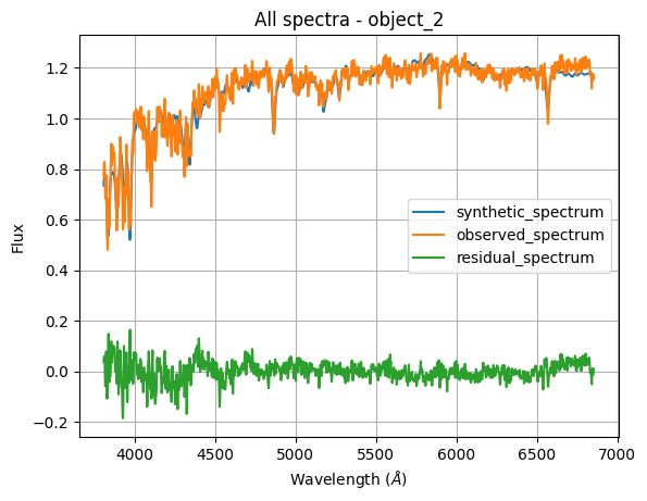
Plotting all spectra

star_object_2.plot()

<Axes: title={'center': 'All spectra - object_2'}, xlabel='Wavelength ($\\AA$)', ylabel='Flux'>

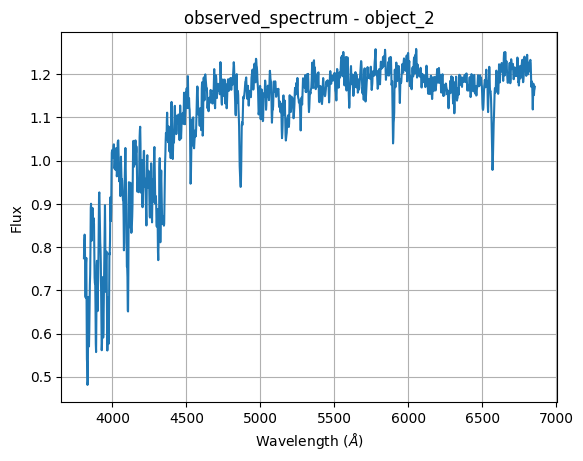
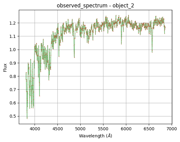
Single spectrum plot

star_object_2.plot.single('observed_spectrum')

<Axes: title={'center': 'observed_spectrum - object_2'}, xlabel='Wavelength ($\\AA$)', ylabel='Flux'>

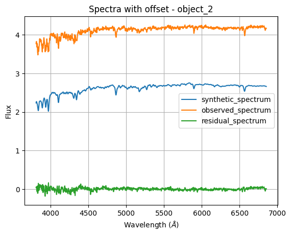
Splited spectra

star_object_2.plot.split(1.5)

<Axes: title={'center': 'Spectra with offset - object_2'}, xlabel='Wavelength ($\\AA$)', ylabel='Flux'>

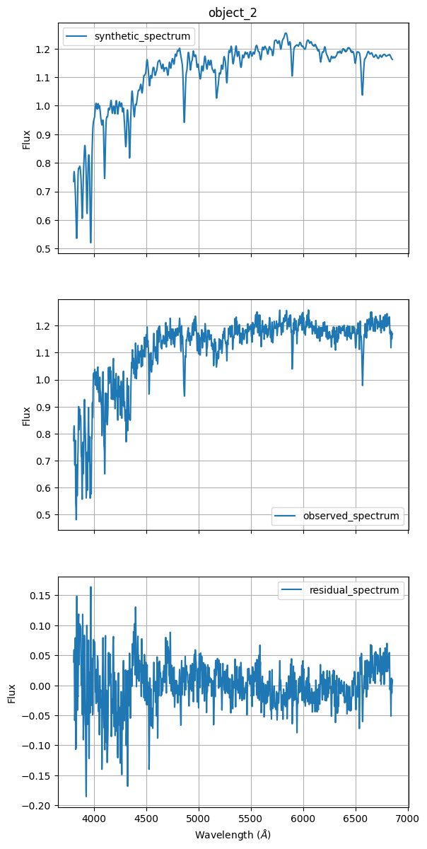
Subplotting all spectra

star_object_2.plot.subplots()

array([<Axes: title={'center': 'object_2'}, ylabel='Flux'>,
       <Axes: ylabel='Flux'>,
       <Axes: xlabel='Wavelength ($\\AA$)', ylabel='Flux'>], dtype=object)

Comparing plots

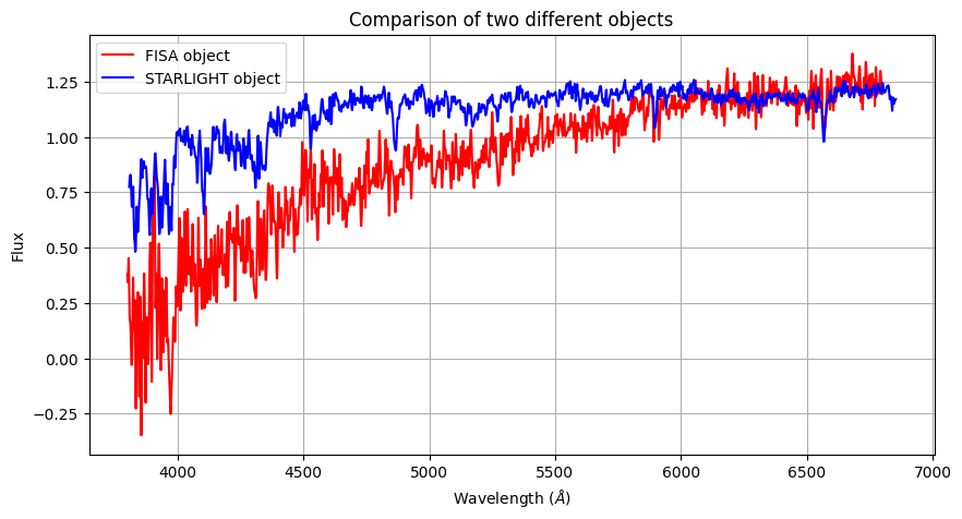
In astronomical analysis is important to compare the spectrum and is very simple to make it using the tools from Spectuils and Matplotliblibraries. First you could save the spectrum in new variables:

plt.figure(figsize=(10, 5))
star_object_1.plot.single('Observed_spectrum', label="FISA object", color='red')
star_object_2.plot.single('observed_spectrum', label="STARLIGHT object", color='blue')

plt.title("Comparison of two different objects")
plt.legend()
plt.show()

Setting your preference in plots

You can set your personal configuration plot. Plots are based on the Matplotlib library; hence, its characteristics may be used.

star_object_2.plot.single(
    'observed_spectrum',
    color = 'green',
    linestyle = '-',
    linewidth = 1.2,
    marker = '*',
    markersize = 0.7,
    markeredgecolor = 'red',
    alpha = 0.5
)

<Axes: title={'center': 'observed_spectrum - object_2'}, xlabel='Wavelength ($\\AA$)', ylabel='Flux'>

NOTE: All the files used in this tutorial are vailable for you in test directory.